Uncertainty refers to the lack of confidence for each output of a machine learning algorithm. While it’s impossible to create an algorithm that has perfect certainty (i.e. I’m 100% sure this is a dog) we need to understand what generates uncertainty, how to quantify it, and how to reduce it. We want to make sure that models describe as precisely as possible the likelihood of their outcome being wrong or outside a given range of accuracy.
Uncertainty estimation is particularly important for neural networks, which have an inclination towards overconfident predictions. Incorrect overconfident predictions can be harmful in critical use cases such as healthcare or autonomous vehicles.
For safe and informed decisions, the models would not only have to provide an output, but also describe as accurately as possible the level of certainty in their outcomes. This means that the models would be delivering their results accompanied by additional information about their uncertainty, and whether the level of uncertainty is low enough for the output to be trusted. Upon producing an output with a high level of uncertainty, the algorithm can call for further information or input from a human to handle the decision making process.
Types of Uncertainty
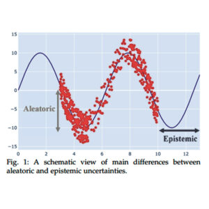
Epistemic Uncertainty
Epistemic uncertainty refers to the model’s uncertainty due to the lack of training data. Epistemic uncertainty is reducible, which means it can be lowered by providing additional data. It’s worth noting that epistemic uncertainty is dependent on how appropriate the data is, which entails relevant, annotated and high-quality data points.
Models are expected to have high epistemic uncertainty when the input data is far away from the training data, and low epistemic uncertainty for data points near the training data. When using a narrow dataset as a baseline, the model would only perform well for inputs within that range. For inputs outside of the training range – but within the scope of the system – the data cannot be categorized correctly due to the model’s lack of knowledge.
Epistemic uncertainty is a high-agenda problem for real-world applications, which may have datasets which are rich in quantity and poor in quality. That’s why epistemic uncertainty can be thought of in terms of the machine learning model’s observability. How much information is the model aware of? Realistically, nobody can provide infinite data or observations, so a model will never be able to reach an epistemic uncertainty of zero. This means that observations from a domain will only be a sample of the existing possibility and always incomplete. Without data or knowledge about the use cases that we’re dealing with, some use cases cannot be solved due to simple lack of awareness that they exist.
Within epistemic uncertainty there is also the issue of bias. Due to a limited training dataset, some of the available data will be biased, so the dataset must be representative of the task or project.
Aleatoric Uncertainty
Compared to epistemic uncertainty, which refers to the lack of data, aleatoric uncertainty refers to the inherent stochasticity of the observations. When data is captured, it is not a perfect representation of reality, but it is contaminated by noise and randomness. Every observation has inherent noise that cannot be controlled, and accumulated, all the noise across observations add up to the model’s aleatoric uncertainty.
While epistemic uncertainty can be reduced with additional observations, aleatoric cannot. Additional data will also include noise captured at the moment of the observation. This type of uncertainty is not a property of the model, but rather is an inherent property of the data distribution, and as such, irreducible. That’s why aleatoric uncertainty is also known as data uncertainty. It can be captured by probabilistic classification and regression models as a consequence of maximum likelihood estimation.
Consider a photograph of a flower. Regardless of how many photographs are taken, there will always be objects in the background, digital noise, dust particles, and different types of lighting. The flower cannot be simply captured by itself without the environment it lives in or without quality degradation when converting analog signal into digital data.
If our scope is making measurements of the flower and storing them as text rather than an image, an observation will store data that describes the object. For example, relevant characteristics can be the species of the flower, its dimensions, color and other similar characteristics. These data points can differ from one flower to another flower of the same species, so there is a degree of variability or randomness. There is no platonic ideal of what objects are supposed to be, and aleatoric uncertainty captures the natural randomness and variability of the world.
One way to estimate aleatoric uncertainty is by using data augmentation during the testing phase. Data augmentation has been typically used to obtain additional training samples by applying transformations such as image flipping, cropping, rotating, scaling, elastic deformations, to create a subset of samples. By generating several augmented examples per test case via data augmentation, we can obtain predictions and use them to estimate uncertainty.
Prediction Uncertainty
Prediction uncertainty is a useful concept which is the conveyed uncertainty in the model’s output calculated by summing together the epistemic uncertainty and aleatoric uncertainty.
Categorizing Uncertainty in a ML Project
Aleatoric and epistemic uncertainty are characteristics of the training data. However, a more practical approach to understanding uncertainty in the context of a machine learning project needs to look at the following – How well does the ML model describe the function it approximates? How suitable is the available data for the application? What is the context in which the model will be deployed? 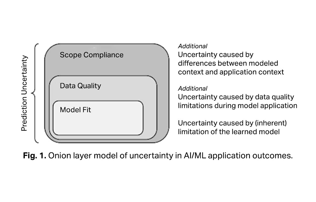
Model Fit Uncertainty
Machine Learning models do not learn to produce real functions, but just empirical approximations of the real relationship between the model input and its outcome. As an approximation, the accuracy of the model’s output is limited by the model’s parameters, hyperparameters, input variables, and available data points. This is often summarized a in an aphorism by George Box:
All models are wrong but some are useful
Uncertainty caused by fitting deficits is commonly measured by the error rate. It is calculated when spitting the cleaned data into a training dataset and a test set. There are two important underlying assumptions regarding uncertainty caused by model fit:
- The model is built and applied on a dataset of consistent quality
- The model is deployed in a context that is adequately represented by the test dataset. This must be true for the cleaned dataset from which the test data is randomly selected
The average uncertainty caused by model fit can be measured using standard model evaluation approaches, which are applied on the training and test data. This will give us the lower boundary approximation of the remaining uncertainty. We must always expect some level of model fit uncertainty due to both the noise in the observations and incomplete coverage of the domain – aka aleatoric and epistemic uncertainty. This will result in imperfect predictions, such as predicting a quantity in a regression problem that is quite different to what was expected, or predicting a class label that does not match what would be expected.
Data Quality Uncertainty
As aleatoric uncertainty refers to the inherent noise in all observations, it cannot be reduced. However, it is different from the quality of a dataset. For example, while all photographs have background objects and other types of noise – which is the aleatoric uncertainty – data quality refers to how well the image is captured. This can include the resolution of an image, clarity, framing of the object, lack of glare and blur, and the like. It also considers the captured objects themselves to be relevant and varied enough for the applications.
The level of certainty in the outcome of an artificial intelligence model is directly proportional to the quality of the training and input datasets. Data quality uncertainty can be seen as the delta between the quality of the cleaned data and the data on which the model is currently being applied. The model’s confidence can decrease when the quality of the input data is lower than the training data. For example, in a computer vision algorithm, a lower resolution camera or a camera with damaged lenses can increase the level of uncertainty.
The impact of data quality uncertainty can be lowered in cases whether the model will be applied with data of lower quality than the cleaned training data. This is done by extending the standard model evaluation procedures with specialized setups that investigate the effect of different quality issues on the accuracy of the outcomes. To do this, data quality has to be quantified and measured not only to annotate raw data with quality information during data preparation, but also to measure the current quality of the data after the model is deployed.
Scope Compliance Uncertainty
Most ML models are built for specific use cases, and whenever used outside of their intended purpose, then their outcomes can become unreliable. In the context of autonomous vehicles, the output of a self-driving machine learning model would be considerably affected if the model was trained and tested for driving on the right hand side, and then used in a left-hand side driving context. Similarly, if the model is trained with data from California, with wide and sunny roads, and used in Scotland, with narrower and lower visibility roads, the model’s uncertainty
To detect and decrease scope compliance uncertainty, we recommend analyzing these common scenarios:
- Determine whether the model can be applied outside the intended scope by monitoring relevant context characteristics and compare the results with the boundaries of the intended scope.
- To determine whether the raw dataset might not be representative of the intended scope, annotate the raw data with context characteristics (e.g., GPS location, velocity, temperature, date, time of day) in order to compare its actual and assumed distribution in the intended scope.
How to Measure Uncertainty
Assigning a level of confidence to model predictions is a major challenge for getting deep learning algorithms deployed in production. Two of the most documented techniques for uncertainty quantification are deep Bayesian neural networks and sparse Gaussian processes. These have some limitations, such as deep Bayesian neural networks suffering from a lack of expressiveness. More expressive models such as sparse Gaussian processes, capture only the uncertainty from the higher-level latent space, making underlying the deep learning model to lack interpretability and ignore uncertainty from the raw data.
We present three other efficient techniques for measuring uncertainty, namely the Monte Carlo dropout, Deep Ensembles, and Deep Bayesian Active Learning.
Monte Carlo Dropout
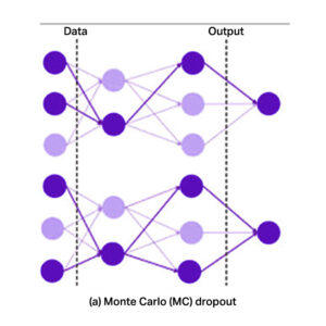
Dropout is an effective technique that has been widely used to solve overfitting problems in DNNs. As a regularization technique during the training process, dropout randomly drops some units of neural network at a certain probability during a forward pass through the network to avoid them from co-tuning too much. Usually, these dropout layers are disabled after training to not interfere with the forward pass on a new data point. To obtain a model’s uncertainty on classifying an image using MC dropout, you would run the prediction multiple times and analyze the different outputs generated by the multiple forward passes.
Deep Ensembles
While Monte Carlo dropout uses one model and makes multiple predictions with deactivated layers, Deep Ensembles use multiple models to enhance predictive performance. These models need to be of the same type, have randomized initial weights and get trained on the same data. To obtain the model’s uncertainty on a given image, it is passed through each of the models in the ensemble and its predictions are combined for analysis. Deep ensembles, compared to Markov Chain Monte Carlo (MCMC) and Bayesian Neural Networks, can be more computationally effective.
Deep ensembles are applied to get better predictions on test data and also produce model uncertainty estimates when models are provided with out of distribution data (OOD). The success of ensembles depends on the variance-reduction generated by combining predictions that are prone to several different types of errors. The improvement in predictions is achieved by utilizing a large ensemble with numerous base models. The ensembles also generate distributional estimates of mode uncertainty.
Deep Bayesian Active Learning (DBAL)
Active learning (AL) methods learn from unlabeled samples by querying an oracle, which work well for a variety of tasks, but lack the scalability to deal with high-dimensional data such as images. This is due to the difficulty of defining the right acquisition function. Acquisition functions are the conditions on which the sample is most informative for the model.
To address this, Bayesian deep learning can represent the uncertainty and then combine the result with the deep active learning acquisition function to probe for the uncertain samples in the oracle. The result is Deep Bayesian Active Learning (DBAL), and it can help an AL framework deal with high-dimensional data problems. DBAL uses batch acquisition to select the top samples with the highest Bayesian Active Learning by Disagreement (BALD) score.
The idea in BALD is to find examples for which many of the different sampled networks are wrong about. The objective is to find the image that maximizes the mutual information between the model output, and the model parameters. To keep only images where the models disagree on, we look for images that have high entropy in the average output and then penalize images where many of the sampled models are not confident about.
Error Calibration
Confidence calibration or optimization refers to the problem of predicting probability estimates representative of the true correctness likelihood. A calibrated output means that the output represents the true probability. For every 100 predictions with a confidence of 0.8, a calibrated output means that 80 samples to be correctly classified. An uncalibrated output would mean that for a 0.8 confidence score, the model would overshoot or undershoot around the mark, such as 70 samples correctly classified rather than the 80 expected. If the confidence estimates are well-calibrated, we can trust the model’s predictions when the reported confidence is high and resort to a different solution when the confidence is low.
Calibration is an orthogonal concern to accuracy, which means that a network’s predictions may be accurate and yet miscalibrated, and vice versa. It’s worth noting that the pseudo-probability of the predicted class almost always overestimates the actual probability of getting a correct answer. For example, if the largest pseudo-probability is 0.9, the algorithm will correctly classify 90 out of 100 data points, but a rather lower rate of 70 or 80 correct predictions. This over-estimation can be measured with techniques such as temperature scaling that modify a neural network so that the output pseudo-probabilities more closely reflect the probability of a correct prediction.
Expected calibration error (ECE) is a metric that compares neural network model output pseudo-probabilities to model accuracy. ECE values can be used to calibrate a neural network model such that output pseudo-probabilities more closely match actual probabilities of a correct prediction.
In contrast to ranking, calibration looks at the actual value of the estimated confidence individually, and tests whether the estimates are over- or under-confident. To measure calibration, a calibration plot was created by splitting the mean maximum Softmax probabilities into 10 bins and calculating the accuracy over each bin. A perfectly calibrated model outputs probabilities that match up with the accuracy and would therefore lie on the diagonal. Probabilities above or below the diagonal are referred to as over-confident or under-confident, respectively. Calibration was measured using the Expected Calibration Error (ECE), which quantifies the difference on the calibration plot between the model’s confidence and the perfect diagonal.24
Miscalibration often stems from increased model capacity and lack of regularization. With model capacity of neural networks having increased considerably over the past few years, we can now expect to see networks with hundreds, if not thousands of layers and hundreds of convolutional filters per layer. This is because algorithms with very deep or wide models are able to generalize better than smaller ones, while also fitting the training set easier. Increased depth and width seems to reduce classification error, but negatively affect model calibration.
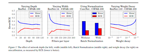
The far left figure varies depth for a network with 64 convolutional filters per layer, while the middle left figure fixes the depth at 14 layers and varies the number of convolutional filters per layer. Though even the smallest models in the graph exhibit some degree of miscalibration, the ECE metric grows substantially with model capacity. During training, after the model is able to correctly classify (almost) all training samples, NLL can be further minimized by increasing the confidence of predictions. Increased model capacity will lower training NLL, and thus the model will be more (over)confident on average.
Another measure of the quality of predictive uncertainty concerns the generalization of the predictive uncertainty to domain shift (also referred to as OOD – out-of-distribution examples). This measures whether the network is aware of what it knows. For example, if a network trained on one dataset is evaluated on a completely different dataset (see the aforementioned section on Scope Compliance), then the network should output high predictive uncertainty as inputs from a different dataset would be far away from the training data. Well-calibrated predictions that are robust to model misspecification and dataset shift are more suitable to be deployed in critical contexts.
Uncertainty Estimation Use Cases
Uncertainty estimation is used to solve the problem of overly confident predictions that are common for deep neural networks. A wrong answer is not necessarily problematic, but a wrong answer with high confidence is an issue, especially for critical applications. Without uncertainty estimation, it is highly unlikely that we’ll see deployment of deep learning applications in critical and large scale real-world systems.
As such, any state-of-the-art machine learning algorithms must not only generate an output, but must also improve the application’s robustness by providing additional information alongside the output, such as a level of confidence in the prediction, whether the level of confidence is accurate – i.e. calibrated – and whether the confidence level is enough to act upon the output.
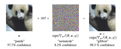
In a real-world environment, uncertainty measurements are necessary as even deviations imperceptible to the human eye may for classification tasks or pattern recognition may result in incorrect outputs. For example, the fast gradient sign method adds a tiny bit of noise to an image and creates an adversarial example. Often, neural networks misinterpret and misclassify this adversarial example with an even higher confidence score than before, while the image appears to a human to be identical.
As such, the below section will describe why uncertainty estimation is applicable for various applications, such as computer vision, image classification, natural language processing, and all their subsets.
Autonomous Vehicles Uncertainty Estimation
Perhaps one of the most obvious use cases for uncertainty estimation is within the autonomous driving industry. By analyzing camera and sensor data in realtime, a self-driving algorithm must determine whether it can accurately detect and understand objects, paths and obstructions. If the camera input does not offer a high enough degree of confidence to accurately identify presence or absence of immediate obstructions, the car should rely more on the output of other sensors for braking, such as Lidar and radar.
Semantic segmentation is an important tool for visual scene understanding and a meaningful measure of uncertainty. Monte Carlo sampling with dropout at test time can generate a posterior distribution to predict pixel wise class labels with a measure of model uncertainty. Uncertainty estimation can help us trust the semantic segmentation output. For instance, a system on an autonomous vehicle may segment an object as a pedestrian, but should also provide the model uncertainty with respect to other classes such as street sign or cyclist in order to consolidate behavioral decisions.
For image segmentation, a 2016 study showed that uncertainty for semantic segmentation in urban remote sensing images can be computed using convolutional neural networks and Monte Carlo dropout. Model uncertainty is higher at object boundaries and in regions where the model is misclassified, which means that pixels with high model confidence are classified correctly more often. When pixels with higher uncertainty were removed, classification accuracy increased. Uncertainty maps are a good measure for the pixel-wise uncertainty of the segmented remote sensing images.
Healthcare Uncertainty Estimation
Healthcare is a ripe industry for machine learning-based classification, especially image classification. Automated image analysis has been around since the first digital images, with sequential application of low-level pixel processing (region growing, edge and line detector filters) and mathematical modeling (fitting lines, ellipses and circles) to build compound rule based systems that solved specific tasks. Examples include active shape models, atlas, concept of feature extraction and use of statistical classifiers.
There is a shift from systems that are entirely devised by humans to systems that are trained by computers utilizing example data from which feature vectors are derived. Computer algorithms establish the optimal decision boundary in the high-dimensional feature space.
With high stakes in terms of ethics, treatment and money, uncertainty estimation is critical in medicine, and the complexity of the issue imposes progressively more complex models. Although deep learning methods have achieved outstanding performances in medical image analysis, most of them have not been employed in extremely automated disease monitoring systems due to lack of reliability of the model.
In medical diagnostics the image registration tasks entails “stitching” together images obtained from scans such as MRI or CT scans. This is a challenging task as images might be taken at different points in time, and a patient’s movement due to breathing for example could mean that the images would not be aligned. Therefore, there’s an inherent uncertainty in the reconstruction process. A model can have high uncertainty when stitching MRI brain scans when there are shape changes in the anterior edge of the ventricle and the posterior brain cortex due to blood flow at different points in time.
Natural Language Processing Uncertainty Estimation
To understand human language, deep learning approaches such as continuous space methods and deep neural networks have inferred language patterns from the huge amounts of real world data and attempt to make accurate predictions about any new data. The acquisition of reliable information from texts is difficult due to the context in which language is used. Uncertainty is a significant linguistic incident that can encompass everything from lack of information, to ambiguity, lack of clarity and context-dependent subtleties in text. Generally, uncertainty for natural language processing can be thought of as a lack of information, making a text’s reliability or truth value difficult to be determined with confidence.
Distinguishing between true and false statements is one of the most important activities for NLP applications. An algorithm needs to recognize linguistic cues of uncertainty since the training data and real-world data may be different. In clinical document classification, medical reports can be grouped depending on whether the patient probability suffers, does not suffer or suffers from an ailment.
For machine translation, recurrent neural networks using naive dropout would result in overfitting, whilst using the Bayesian variant of dropout, the model would not overfit and achieve state-of-the-art results on multiple language pairs.
High Frequency Trading
In stock exchanges or other financial institutions, rule-based decision making systems have governed transactions for decades. In this type of complex environment with many dependencies and fragile balance, machine learning applications need high levels of confidence and certainty to be deployed in production. Therefore, we need a validation phase before deploying any high frequency trading algorithms to determine how the application will behave in a simulated environment. Second, the algorithm needs a system to deal with low-confidence or high uncertainty instances. A simple solution is to implement humans-in-the-loop. For an instance where a ML algorithm does not have high enough certainty to act, the input would be passed onto a human operator and the ML algorithm would move onto other instances.
Conclusion
Uncertainty is a natural quality of any machine learning problem. It is tied to not only the training and real world data, but also to the ML model and any human biases that get baked into the algorithm. Despite the fact that some level of uncertainty will always be present, there are multiple ways in which this can be identified, calculated and reduced. Especially for mission-critical systems, developers need to develop failover systems that can ensure machine learning systems deployed in production can deliver >99% SLAs.